Introduction

Opposed to block codes, convolutional codes don’t divide data bits into blocks. In convolutional codes, data bits are still in continuous sequence. In some occasions, convolution codes maybe more convenient than a block code, because it generates redundant bits and corrects errors continuously.

Convolutional code can be marked by (n, k, K), which means for every k bits, there are an output of n bits and K is called constraint length. Basically, convolutional code is generated by passing the information sequentially through a series of shift registers. K stands for the number of the shift registers. Because of the shift registers, convolutional code has memory, the current n-bit output depends not only on the value of the current block of k input bits but also on the previous K-1 blocks of k input bits. 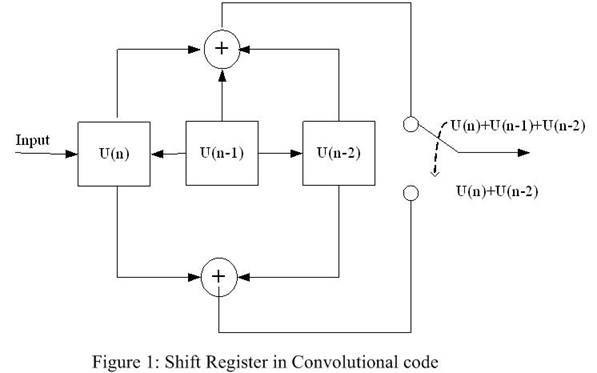So, the current output of n bits is a function of the last K×k bits. As shown in Figure, 3 most recent bits have used and two possible outputs are generated. Typically, n and k are very small number. Here, the figure shows (2,1,3) codes.

For any (n,k,K) code, the shift register keeps most recent K×k input bits. Starting from initial states, the encoder produces n output bits, after that, the oldest k bits from the register are discarded and k new bits are shifted in. For any given input of k bits, there are different functions that map k bits into n output bits. What kind of functions is used depends on the history of the last (K-1) input blocks. Since the convolutional encoder can be identified as a K-memory, n output machine, it can be expressed as a 0-1 sequence, which is called generator sequence g(.). With 2 output in Figure 1, there are 2 sequences:. Then the generator matrix is defined as:

,

So, the output of the encoder is

,

Where, u is the input.

Viterbi decoder algorithm is a kind of maximum likelihood decoder and the most popular decoder for convolutional codes. The easily way to introduce Viterbi algorithm is using state diagram of the encoder, namely trellis diagram.

Figure 2 trellis diagram of sample rate 0.5, constraint length K = 3 convolutional encoder^[1]

Figure 2 is a simple example of a sample rate 0.5 and constraint length 3 convolutional encoder. At start time, the system is at state 00. With different input, the state will transient to different state. At each time step, there is only one bit input, either be 0 or 1. So the state transient paths will separate to two at each time step. The solid line means with input signal 1 and the dashed line is with input signal 0. At last it will return to the state 00 (because the registers are all zeros), and there will multiple paths from the start state to the end state.

The key idea of Viterbi algorithm is to find the most likelihood sample path with the received codes. The formal description of Viterbi algorithm can be found at [2]. An error metric is setup for each path. When decoder receives a data bit, it will compute the partial metric for the single path entering each state, and store the path with its metric. At next time step, re-compute the partial metric for all paths entering a state by adding the accumulated error metric.

For each state, decoder only stores the path with the largest metric and eliminates all other paths. Figure 3 is a simple example, where the at time unit 5, the state 11 has the smallest error, which means the path to state 11 is most likely correct path.

Figure 3 Trellis diagram with accumulated error metric^[1]

At last the decoder will get a most likelihood path from initial state to ended state. Tracing back the sample path, decoder can decide the data from each state transient step.

Detailed algorithm and performance analysis are discussed at [2]. Also [1] is a very nice and detailed tutorial for convolutional encoder and Viterbi decoder.

Usage

The program is developed with Java applet. Basically, the implementation involves three steps: Encoder, Error adding, Decoder.

· Encoder

Constraint length (K) and message length is available for adjusting. Considering the limitation of displaying, K is set to range from 3 to 7. The codeword in convolution coding is usually pretty long. User will be able to choose either to manually type data stream in Hex (user generate) or allow program to randomly generate data stream (randomly generate). If “randomly generator” is selected, upon K and data length being settled, the program will randomly generate a data stream and encoder it into codeword.
With the “random gen” or “user gen” button being clicked, the original signal, convolutional and its generator sequence (details have been discussed above) will be displayed. Meanwhile, the data stream and codeword will be show the plot graph underneath.

· Error Adding

Error Adding will be implemented in term of two styles: error inferred by probability and fixed-length error.

· Error inferred by probability

In this category, user will be allowed to set “failure probability for each bit”, and the error bits will be applied according to the probability.

· Fixed-length error

In this category, user is allowed to decide number of errors that will happen to codeword. Besides, two error-assignment forms will be available to be selected:

Random: The faulty bits will be randomly selected from the codeword;

Burst: The faulty bits will be consecutive, and user is allowed to set start position for burst error. In random styles, the start position will be set to “-1”, meaning not available for adjustment. If the start position that user set exceeds the length of the codeword, the program will coerce the start position back to signal range. It is well know that burst errors are hard for normal other error correction codes to deal with. But user will find burst or separate errors make no difference for convolutional code, which is an advantage of such code. When “adding error” is clicked, the receiving code with error bits will be displayed. Meanwhile, corresponding receiving code will be shown in the plot graph. On the receiving curve, a red “E” will appear on the error bit.

· Decoder

The decoder will be triggered by user clicking the “decode”. The decoder will give the results of error corrections, including:

· decoded signal;

· The number of corrected errors;

· The text message, which indicates whether all the error bits have been corrected.

· The trellis diagram: it shows the maximum likely-hood path from Viterbi algorithm, which is identical to the one in Figure 3 and will be shown under the plot graph.

The decoded signal will also be shown in the plot graph. When the number of errors exceeds the error-correction capability decoder will fail to correct all the errors. In that case, some of “E”s will be left to indicate that some errors are still there.

Reference:

[1] Lin, Shu, and Costello, Deniel, “Error Control Coding: Fundamentals and Applications”, Prentice-Hall Inc., 1983.

[2] Tutorial of Convolutional Codes: http://home.netcom.com/~chip.f/viterbi/algrthms.html#algorithms