Empirical Lake Model for Phosphorus with Uncertainty[1]

Importance of Phosphorus on Lake Quality

Lake Nutrient Classification

Phosphorus Conc. (mg/L)	Trophic State	Lake Use
<0.010	Oligotrophic	Suitable for water-based recreation and propagation of cold water fisheries, such as trout. Very high clarity and aesthetically pleasing. Excellent as a drinking water source.
0.010 - 0.020	Mesotrophic	Suitable for water-based recreation but often not for cold water fisheries. Clarity less than oligotrophic lake.
0.020 - 0.050	Eutrophic	Reduction in aesthetic properties diminishes overall enjoyment from body contact recreation. Generally very productive for warm water fisheries. High TOC and algal tastes & odors make these waters less desirable as a water supply.
> 0.050	Hypereutrophic	A typical "old-aged" lake in advanced succession. Some fisheries, but high levels of sedimentation and algae or macrophyte growth may be diminishing open water surface area. Generally, unsuitable for drinking water supply.

The Phosphorus Lake Model

This model is based on a simple mass balance with terms for loading (W), settling, and outflow. There is no spatial, or temporal resolution.

Dividing both sides by the surface area (A_s) gives:

where, H is the lake depth, L is the areal loading (W/A_s) and q_s is the overflow rate (Q/A_s). At steady state (dP/dt =0), the solution becomes:

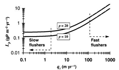
Based on data from 47 northern temperate lakes included in EPA's National Eutrophication Survey, the settling velocity (in m/yr) was found to be an empirical function of the overflow rate[2]:

so substituting this into the steady state model above, we get:

where:

P = mean annual total phosphorus concentration (g-P/m³ or mg-P/L)

L = mean annual areal phosphorus loading (g-P/m²-yr)

q_s = mean annual areal water loading or overflow rate (m/yr) = Q/A_s

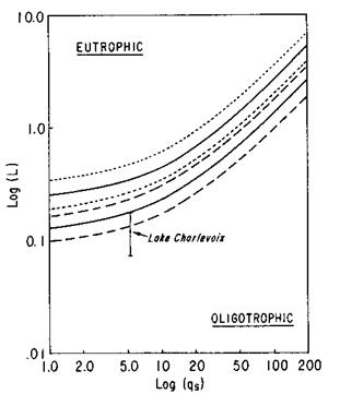
This model was developed from lakes with phosphorus concentrations in the range of 0.004-0.135 mg/L, phosphorus loadings of 0.07-31.4 g-P/m²-yr, and overflow rates of 0.75-187 m/yr. It should not be used for lakes whose characteristics are outside of this range. When used properly, the log transform of the model has an estimated error (s_mlog) of 0.128. This value was determined from comparison of observed and predicted phosphorus concentrations in the 47 lakes. Therefore, considering error, the model can be written as:

From Chapra (pg 538)

from: Reckhow, 1979

Determination of Areal Water Loading (overflow rate)

q_s = Q/A_s

If Q is not directly measurable from inflow or outflow, then it can be estimated from:

Q = (A_d x r) + (A_s x Pr)

where:	qs =	areal water loading (m/yr)
	Q =	inflow water volume to lake (m^3/yr)
	Ad =	watershed area (land surface) (m^2)
	As =	lake surface (m^2)
	r =	total annual unit runoff (m/yr)
	Pr =	mean annual net precipitation (m/yr)

Data Collection

· Determine total drainage area (A_d) from a GIS database, or USGS maps, using a polar planimeter, or cut paper with squares.

· Estimate the surface area of the lake (A_s). This may also be done by GIS or planimetry using a USGS map, or the cut paper method.

· Estimate annual runoff (r) which is usually expressed in meters/year. This information is generally available from the USGS.

· Determine average annual net precipitation (Pr), also expressed as meters/year. This information can usually be obtained from the USGS or the US Weather Service.

Determination of Areal Loading with Uncertainty

First determine total phosphorus mass loading (W):

W = (Ec_f x Area_f) + (Ec_ag x Area_ag) + (Ec_u x Area_u) + (Ec_a x A_s)

+ (Ec_st x #capita-yrs x [1-S.R.]) + PSI

where:	Ecf =	export coefficient for forest land (kg/ha-yr)
	Ecag =	export coefficient for agricultural land (kg/ha-yr)
	Ecu =	export coefficient for urban area (kg/ha-yr)
	Eca =	export coefficient for atmospheric input (kg/ha-yr)
	Ecst =	export coefficient to septic systems impacting the lake (kg/(capita-yr)-yr)
	Areaf =	area[3] of forested land (ha)
	Areaag =	area of agricultural land (ha)
	Areau =	area of urban land (ha)
	As =	surface area of lake (ha)
	#capita-yrs	number of capita-years in watershed serviced by septic tank impacting the lake
	S.R. =	soil retention coefficient (dimensionless)
	PSI =	point source input (kg/yr)

Data Collection

· Estimate land use drainage areas (forested, agricultural, urban). This information may be available from local planning agencies, otherwise it may be obtained from GIS data. For future projections, high and low estimates are needed for assessment of uncertainty

· Choose Export Coefficients for each category. Ranges should be selected for the major sources (often all but precipitation). Choice depends on characteristics of watershed as compared to those previously studied, for which there already exists export coefficients. Other factors may play a role such as the use of phosphate detergents (will impact Ec_st).

Some Non-specific Phosphorus Export Coefficients

Source	Symbol	Units	High	Mid-range	Low
Agricultural	Ecag	kg/(ha-yr)	3.0	0.4-1.7	0.10
Forest	Ecf	kg/(ha-yr)	0.45	0.15-0.3	0.02
Precipitation	Eca	kg/(ha-yr)	0.60	0.20-0.50	0.15
Urban	Ecu	kg/(ha-yr)	5.0	0.8-3.0	0.50
Input to septic tanks	Ecst	kg/(capita-yr)	1.8	0.4-0.9	0.3

· Estimate SR: This is a number between 0 and 1 that indicates how well the soil and associated plants take up phosphorus. When it is low more of the phosphorus reaches the lake. Factors to consider include:

· phosphorus adsorption capacity

· natural drainage

· permeability

· slope

· Estimate number of capita-years on septic systems impacting lake: This requires some judgment, but usually a strip of about 20-200 m wide surrounding the lake is considered the zone of influence. All septic systems within this zone would be counted in the following calculation:

Total # of capita-years

=

average # of persons per living unit

X

# days spent at unit per year /360

X

# of living units within zone of influence

· Estimate Point source inputs: possibly from NPDES permits

· Now determine high, low and most likely estimates of W using above equation. These are obtained from high, low and most likely estimates of the various input parameters (note that the low value of S.R. should go with the high estimate of W, and vice versa).

Next determine areal loading (L)

· From these three estimates of W, calculate the high, most likely and low estimates for annual areal phosphorus loading

L = W/A_s

Calculation of Lake Phosphorus Level and Confidence Intervals

Evaluate the three estimates of phosphorus concentration

Estimate Prediction Uncertainty (s_T)

This requires that the model error be appropriately combined with the uncertainty inherent in the model terms. This is done on log transforms of the model results, using standard error propagation techniques.

Model Error

· positive and negative model errors are calculated separately and not presumed equal.

s_m+ = antilog[logP_ml + s_mlog] - P_ml

s_m- = antilog[logP_ml - s_mlog] - P_ml

Error in Model Terms

s_L+ = (P_(high) - P_(ml))/2

s_L- = (P_(ml) - P_(low))/2

Overall Error

s_T+ = [(s_m+)² + (s_L+)²]^0.5

s_T- = [(s_m-)² + (s_L-)²]^0.5

Confidence Intervals

· The intervals are 55% for 1 prediction error, and 90% for 2 (based on a modification of the Chebyshev inequality).

55% confidence interval:	(P(ml) - sT-) < P < (P(ml) + sT+)
90% confidence interval:	(P(ml) - 2sT-) < P < (P(ml) + 2sT+)

The Lake Higgins Example

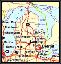
This lake is located in the northern section of Michigan's lower peninsula. It is a deep, cool, oligotrophic lake with a well oxygenated hypolimnion. Its maximum depth is 41 m, and it has a mean depth of 15 m.

Determination of Areal Water Loading (overflow rate)

Ad =	87.41 x 10^6 m^2
As =	38.4 x 10^6 m^2
r =	0.2415 m/yr
Pr =	0.254 m/yr

Q = (A_d x r) + (A_s x Pr)

Q = 30.863 x 10⁶ m³/yr

q_s = Q/A_s

q_s = 0.804 m/yr

Determination of Areal Loading with Uncertainty

Land Use	Area (ha)
Agricultural	16
Forest	8347
Urban	378

· forested land: mostly coniferous

· agricultural land: limited, mostly grazing and pasture

· urban areas: mainly residential and recreational, all are on septic systems

· septic systems: phosphorus-based detergents are banned in Michigan, so this value will be low

· precipitation: value will also be low because of low agricultural and industrial inputs in the watershed which contribute to airborne phosphorus

Phosphorus Export Coefficients

Source	Symbol	Units	High	Most Likely	Low
Agricultural	Ecag	kg/(ha-yr)	1.3	0.40	0.20
Forest	Ecf	kg/(ha-yr)	0.30	0.20	0.10
Precipitation	Eca	kg/(ha-yr)	0.50	0.30	0.15
Urban	Ecu	kg/(ha-yr)	2.70	0.90	0.35
Input to septic tanks	Ecst	kg/(capita-yr)	1.0	0.6	0.3

· Estimation of SR: Higgins Lake is situated in an area of sandy/gravel soils for moraines and till plains, which tend to permit rapid infiltration and transmission of water. Furthermore, neighboring Houghton Lake is known to be surrounded by soils of low phosphorus adsorbing capacity. As a result a relatively low set of SRs were chosen:

Soil Retention Coefficient

Symbol	Units	High	Most Likely	Low
S.R.	unitless	0.50	0.25	0.05

· Estimate number of capita-years on septic systems impacting lake: Only lakeside dwellings were counted:

Total # of capita-years

=

3.5 persons/unit

X

60 days spent at unit per year /360

X

1000 living units within zone of influence

Total # of capita-years = 575.3

· No point source inputs to Higgins Lake

· Now determine high, low and most likely estimates of W

W = (Ec_f x Area_f) + (Ec_ag x Area_ag) + (Ec_u x Area_u) + (Ec_a x A_s)

+ (Ec_st x #capita-yrs x [1-S.R.]) + PSI

W_(high) = (0.30 x 8347) + (1.30 x 16) + (2.7 x 378) + (0.50 x 3840)

+ (1.0 x 575.3 x [1-0.05]) + 0

W_(ml) = (0.20 x 8347) + (0.40 x 16) + (0.90 x 378) + (0.30 x 3840)

+ (0.6 x 575.3 x [1-0.25]) + 0

W_(low) = (0.10 x 8347) + (0.20 x 16) + (0.35 x 378) + (0.15 x 3840)

+ (0.3 x 575.3 x [1-0.50]) + 0

· From these three estimates of W, calculate the high, most likely and low estimates for annual areal phosphorus loading

L = W/A_s

Summary of Results

Parameter	High	Most Likely	Low
W	6012.04 kg/yr	3426.9 kg/yr	1632.5 kg/yr
L	0.157 g/m^2-yr	0.089 g/m^2-yr	0.043 g/m^2-yr
P	0.0125 mg/L	0.0071 mg/L	0.0034 mg/L

Calculation of Lake Phosphorus Level and Confidence Intervals

· using the model, determine the three estimates of P:

for results, see table above.

Estimate Prediction Uncertainty (s_T)

Model Error

s_m+ = antilog[logP_ml + s_mlog] - P_ml

s_m+ = antilog[log0.0071 + 0.128] - 0.0071

s_m+ = 0.0024 mg/L

s_m- = antilog[logP_ml - s_mlog] - P_ml

s_m- = antilog[0.0071 - 0.128] - 0.0071

s_m- = 0.0015 mg/L

Error in Model Terms

s_L+ = (P_(high) - P_(ml))/2

s_L+ = (0.0125 - 0.0071)/2

s_L+ = 0.0027 mg/L

s_L- = (P_(ml) - P_(low))/2

s_L- = (0.0071 - 0.0034)/2

s_L- = 0.0019 mg/L

Overal Error

s_T+ = [(s_m+)² + (s_L+)²]^0.5

s_T+ = [(0.0024)² + (0.0027)²]^0.5

s_T+ = 0.0036

s_T- = [(s_m-)² + (s_L-)²]^0.5

s_T- = [(0.0015)² + (0.0019)²]^0.5

s_T- = 0.0024

Confidence Intervals

55% confidence interval:	0.0047 < P < 0.0107
90% confidence interval:	0.0023 < P < 0.0143

---

[1] From Reckhow & Chapra, Engineering Approaches for Lake Management, Volume 1, pp272-291.

[2] From: Reckhow, 1979 [JWPCF 51(8)2123-2128] “Uncertainty Analysis Applied to Vollenweider’s Phosphorus Loading Criterion”

[3] Recall that ha stands for hectare which is equal to 10,000 m².