CHAPTER XXIII
PARAMETRIC STATISTICS
A. INTRODUCTION
In a sample, the true concentration of an analyte can never be determined with absolute certainty. The presence of random error and systematic error causes excursions from the true value. Systematic errors result in a condition known as bias. Bias is characterized by a shift in the data mean away from the true value (historically, the term "accuracy" was also used to describe this quality, however, current usage has given accuracy a broader meaning). A positive bias means that the method tends to overestimate the concentration of the analyte. A negative bias is the result of consistent underestimation. Incomplete recovery of analyte in precipitative gravimetric analysis is an example of a negative bias. Data containing large random errors is said to be imprecise. Precision is a measure of the reproducibility of the data. It says nothing about the proximity to the true value. When data are both precise, and unbiased, they are said to be accurate.
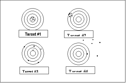
Figure 23.1 presents a target analogy for chemical analysis. Target 1 represents a set of data which show a high degree of precision and very little bias. Such data are therefore, referred to a being accurate, and all of the other targets are inaccurate. Target 2 shows good precision, but a high degree of bias. Target 3 shows little or no bias, but poor precision. Finally, target 4 has both bias and poor precision.
#1 #2 #3 #4

Figure 23.1
Errors in Target Shooting and Chemical Analysis
B. POPULATION STATISTICS
1. Central Tendency
The three most common measures of
central tendency are the mean, median, and mode. The mean, ![]() ,
is simply equal to the sum of the values for all of the observations divided by
the number of observations, n.
,
is simply equal to the sum of the values for all of the observations divided by
the number of observations, n.
![]() (23.1)
(23.1)
The mean is most useful in characterizing the central tendency for measurements that are distributed normally. The sample mean as defined by equation 23.1 is an estimate of the population (true) mean, often represented by . Note that this value, , is not necessarily equal to the true value of the analyte concentration. The discrepancy between and the true concentration is due to systematic error (bias). For highly skewed distributions, the median may be the most appropriate statistic for central tendency. It is obtained by listing all of the observations in ascending order. The median is then the middle value; half the observations being greater in value; and half being less. The mode is the most frequently measured value.
2. Variance and Standard Deviation
The spread of observations about the mean or median is characterized by the standard deviation or variance of the population. Although the true population standard deviation, s, cannot be directly measured, it can be estimated from a finite group of measurements all on the same sample using equation 23.2. This estimate of the population standard deviation called the sample standard deviation is given the symbol, s. It is often more convenient to use the far right-hand term in equation 23.2 to calculate s, however, it is very sensitive to round-off errors. Do not round-off until the value of "s" is obtained.
 (23.2)
Sometimes one is faced with 2 or 3 replicates on each of a number of samples, rather than a large number of replicates on a single sample. In this case standard deviations can be calculated for each by equation 23.2. Then the individual standard deviations can be pooled. This will provide a better estimate of the population standard deviation than any one of the single standard deviations.
 (23.3)
One is commonly confronted with data composed of a set of duplicate analyses on "k" different samples. For this simple case, equations 23.2 and 23.3 can be combined to get equation 23.4, where "d" is the difference between each pair of duplicates.

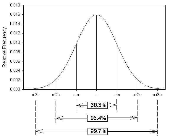
Figure 23.2
Mean and Standard Deviation of Normally Distributed Data
![]() (23.4)
(23.4)
The variance is simply the square of the standard deviation. For a normal or bell-shaped distribution, 68.3% of the observations will fall within 1 standard deviation of the mean, 95.4% within 2 standard deviations and 99.7% within three (see Figure 23.2).
Example 23.1
One large sample of river water is collected and analyzed for total solids and total dissolved solids. Four determinations of each are made using 75mL subsamples. The net weights (in grams) for each are shown below:
|
|
TDS |
TS |
|
#1 |
0.0433 g |
0.0475 g |
|
#2 |
0.0401 g |
0.0461 g |
|
#3 |
0.0498 g |
0.0495 g |
|
#4 |
0.0442 g |
0.0509 g |
What are the mean values for TDS, TS and TSS for this water? What are the standard deviations for the TDS and TS determinations?
First the four values for each parameter must be summed, and then divided by the total number of observation (4). Then the results must be divided by the volume used, to get them in the form of a concentration, preferable in the standard units, mg/L. The mean TSS is then the difference between these two means.
|
|
TDS |
TS |
(TDS)2 |
(TS)2 |
|
#1 |
0.0433 g |
0.0475 g |
0.0018749 |
0.0022563 |
|
#2 |
0.0401 g |
0.0461 g |
0.0016080 |
0.0021252 |
|
#3 |
0.0498 g |
0.0495 g |
0.0024800 |
0.0024503 |
|
#4 |
0.0442 g |
0.0509 g |
0.0019536 |
0.0025908 |
|
= |
0.1774 g |
0.1940 g |
0.0079166 |
0.0094225 |
|
|
0.0444 g |
0.0485 g |
|
|
|
= |
591 mg/L |
647 mg/L |
|
|
![]() =
647-591 mg/L = 56 mg/L (23.E1)
=
647-591 mg/L = 56 mg/L (23.E1)
In order to calculate standard deviations, we first must calculate the sum of the squares of each of the measurements. This has been done above. The standard deviations are simply calculated from equation 23.2 and dividing by the sample volume.
 (23.E2)
 (23.E3)
The results for TDS and TS should be expressed as a mean plus or minus a standard deviation.
TDS = 591 53 mg/L
TS = 647 28 mg/L
PROPAGATION OF ERRORS
1. Multiplication/Division by a Constant
This is a very simple case where the standard error can simply be multiplied or divided by the constant used to adjust the mean. This can only be done when the constant, n, has an insignificant error associated with it as compared to the error (or standard deviation, s) in "x".
n(x s) = nx ns (23.5)
This type of manipulation was performed in Example 23.1 in converting standard deviations from grams (per 75 mL) to mg/L.
2. Addition/Subtraction of Two Numbers with Significant Errors
When two measurements having errors of the same order of magnitude are added or subtracted, the variances can be directly added. This means that the standard deviation or error for the sum/difference is the geometric mean of the original two standard deviations.
![]() (23.6)
(23.6)
![]() (23.7)
(23.7)
3. Multiplication/Division of Two Numbers with Significant Errors
When two measurements having relative errors of the same order of magnitude are multiplied or divided by each other, the relative variances can be directly added. This means that the standard deviation or error for the product/quotient is the geometric mean of the original two relative standard deviations.
![]() (23.8)
(23.8)
 (23.9)
CONFIDENCE INTERVALS
The most commonly used
confidence interval is the 95% confidence for the mean. This gives a range within which you are 95%
certain that the actual mean value (which cannot be directly measured) actually
falls. In order to calculate this
value, one must first calculate the standard error of the mean, ![]() .
.
![]() (23.10)
(23.10)
As
before, n is the number of replicate observations or sets of observations used
to calculate s. This gives you a
measure of the error of your estimate, ![]() ,
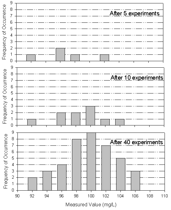
of the true population mean, . Figure 23.3 shows how increasing the number of observations, n,
will improve one's confidence that
,
of the true population mean, . Figure 23.3 shows how increasing the number of observations, n,
will improve one's confidence that ![]() is a good estimate of the true mean.
is a good estimate of the true mean.
The confidence interval is the mean plus or minus the standard error of the mean multiplied by some "t-statistic".
![]() (23.11)
(23.11)
The t-statistic comes from the student-t distribution. It is a function of the number of degrees of freedom and the accepted alpha error. In most cases, the number of degrees of freedom simply equals n-1. One is subtracted because a degree of freedom is lost when the mean is calculated. For a 95% confidence interval, one is willing to accept a 2.5% chance that the mean actually is above the range, and a 2.5% chance that it is below the range. Therefore, the alpha value will be 2.5%.

Figure 23.3
Frequency Histogram of Replicate Determinations of an Analyte
(the true value is 100 ppm)
Table 23.1
Student's t Distribution
|
Degrees of |
Alpha Values |
||||
|
Freedom |
10% |
5% |
2.5% |
1% |
0.5% |
|
1 |
3.078 |
6.314 |
12.706 |
31.821 |
63.657 |
|
2 |
1.886 |
2.920 |
4.303 |
6.965 |
9.925 |
|
3 |
1.638 |
2.353 |
3.182 |
4.541 |
5.841 |
|
4 |
1.533 |
2.132 |
2.776 |
3.747 |
4.604 |
|
5 |
1.476 |
2.015 |
2.571 |
3.365 |
4.032 |
|
6 |
1.440 |
1.943 |
2.447 |
3.143 |
3.707 |
|
7 |
1.415 |
1.895 |
2.365 |
2.998 |
3.499 |
|
8 |
1.397 |
1.860 |
2.306 |
2.896 |
3.355 |
|
9 |
1.383 |
1.833 |
2.262 |
2.821 |
3.250 |
|
10 |
1.372 |
1.812 |
2.228 |
2.764 |
3.169 |
|
15 |
1.341 |
1.753 |
2.131 |
2.602 |
2.947 |
|
20 |
1.325 |
1.725 |
2.086 |
2.528 |
2.845 |
|
inf. |
1.282 |
1.645 |
1.960 |
2.326 |
2.576 |
Example 23.2
What is the standard error of the mean for TSS of the river water from Example 23.1? What is the 95% confidence interval for this number?
First a standard error of the mean must be calculated for each of the two direct measurements, TDS and TS.
![]()
![]()
Next, equation 23.7 may be used directly to propagate these standard errors.

Finally, use equation 23.11 to calculate the confidence interval. The number of degrees of freedom will be 6 (i.e, [nTDS-1]+[nTS-1]=6). The alpha value will be 2.5%.
![]()
OUTLIERS
Outliers may be identified and rejected in one of two ways. First, if there is any evidence, independent of the numerical value of the determination, that the sample was not representative or that some error was committed in the analytical procedure, the data point may be rejected. Second, if the numerical value departs significantly from that of other replicates, the data point may be rejected.
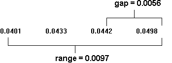
One way of determining if a data is significantly different from other replicates is Dixon's "Q" Test. First the replicate data are arranged in ascending order, X1 to Xn. The "gap" is defined as the difference between the data in question and the next closest data point for data sets up to 10. For replicates that number between 11 and 25, the suspected outlier and the second closest point define the "gap". The "range" is the difference between the highest point and the lowest, including the data point in question. If the replicates number 8-13, the extreme value that is not the suspected outlier is dropped, and the range is calculated using the next most extreme value. If 14-25 replicates are being compared the two most extreme values on the side opposite the suspected outlier are dropped. The Dixon quotient is then the ratio of gap to the range.
![]() (23.12)
(23.12)
This quotient is compared with the appropriate Qs from Table 23.3. In order to pick a Qs one must first decide the level of significance, or the risk one is willing to take for a false rejection. The data point can be rejected, if Q > Qs.
Table 23.2
Calculating Quotients for Dixon's Test
|
# Observations |
Statistic |
Test for High
Value, Xn |
Test for Low Value, X1 |
|
3-7 |
Q10 |
(Xn-Xn-1)/(Xn-X1) |
(X2-X1)/(Xn-X1) |
|
8-10 |
Q11 |
(Xn-Xn-1)/(Xn-X2) |
(X2-X1)/(Xn-1-X1) |
|
11-13 |
Q21 |
(Xn-Xn-2)/(Xn-X2) |
(X3-X1)/(Xn-1-X1) |
|
14-25 |
Q22 |
(Xn-Xn-2)/(Xn-X3) |
(X3-X1)/(Xn-2-X1) |
Example 23.3
Determine if the high value for total dissolved solids on the river water in Example 23.1 is an outlier.
First arrange the data in ascending order. Since n=4, no values are excluded in calculating the gap and range (i.e., the Q10 statistic is used).

Thus, Q10 = 0.0056/0.0097 = 0.58. Choosing an alpha level of 5%, the appropriate Qs is 0.765. Since Q10 is less than this value we cannot reject this value for TDS.
Table 23.3
Values for Dixon's Quotient, Qs
|
|
|
Risk of False Rejection |
|||
|
Statistic |
# Observations |
0.5% |
1% |
5% |
10% |
|
Q10 |
3 |
0.994 |
0.988 |
0.941 |
0.886 |
|
|
4 |
0.926 |
0.889 |
0.765 |
0.697 |
|
|
5 |
0.821 |
0.780 |
0.642 |
0.557 |
|
|
6 |
0.740 |
0.698 |
0.560 |
0.482 |
|
|
7 |
0.680 |
0.637 |
0.507 |
0.434 |
|
Q11 |
8 |
0.725 |
0.683 |
0.554 |
0.479 |
|
|
9 |
0.677 |
0.635 |
0.512 |
0.441 |
|
|
10 |
0.639 |
0.597 |
0.477 |
0.409 |
|
Q21 |
11 |
0.713 |
0.679 |
0.576 |
0.517 |
|
|
12 |
0.675 |
0.642 |
0.546 |
0.490 |
|
|
13 |
0.649 |
0.615 |
0.521 |
0.467 |
|
Q22 |
14 |
0.674 |
0.641 |
0.546 |
0.492 |
|
|
15 |
0.647 |
0.616 |
0.525 |
0.472 |
|
|
16 |
0.624 |
0.595 |
0.507 |
0.454 |
|
|
17 |
0.605 |
0.577 |
0.490 |
0.438 |
|
|
18 |
0.589 |
0.561 |
0.475 |
0.424 |
|
|
19 |
0.575 |
0.547 |
0.462 |
0.412 |
|
|
20 |
0.562 |
0.535 |
0.450 |
0.401 |
PROBLEMS
23.1 Ten replicate measurements for Nitrite-nitrogen were measured on a sample of water from the Azote River (all values are in units of mg/L):
|
0.032 |
0.047 |
|
0.037 |
0.073 |
|
0.031 |
0.039 |
|
0.033 |
0.030 |
|
0.032 |
0.034 |
a. Determine the 95% confidence interval for the mean concentration of nitrite nitrogen based on these measurements. Use the Dixon test to find any outliers (use an alpha value of 5%)
b. Other tests on this water have found the following concentrations for this water:
|
Parameter |
Mean (mg/L) |
95% Confidence Interval (mg/L) |
|
Ammonia-nitrogen |
0.182 |
0.013 |
|
Nitrate-nitrogen |
0.055 |
0.009 |
|
Organic-nitrogen |
0.151 |
0.019 |
Determine the total nitrogen content and its 95% confidence interval.